Quantitative Analysis Tools for Phytosanitary Measures: a Perspective from South America

Ricardo B. Sgrillo
Cocoa Research Center (CEPLAC/CEPEC)
Rod. Ilheus-Itabuna, km 22, 45650-000 Ilheus, BA, Brazil
ricardo.sgrillo@terra.com.br
This paper represents the views of the author and not necessarily those of his country and/or organization.

Presented as invited paper at:

INTERNATIONAL CONFERENCE ON SANITARY & PHYTOSANITARY (SPS) RISK ASSESSMENT METHODOLOGY
"Optimization of SPS Regulatory Tool-Box"
August 9 - 11, 2005
Washington DC

Download Paper (.pdf)

Download Presentation (.pdf)

Summary

This paper presents some concepts and quantitative tools that could be used for the development of phytosanitary regulations for plants and plant products. These concepts could increase biosecurity, reduce unjustified trade barriers and add transparency to the regulation process. Equations are shown that give meaning to the Acceptable Level of Risk concept through which it is established an acceptable probability level for pest introduction. Some aspects regarding application of phytosanitary measures to reduce the probability of pest introductions to an acceptable level, either by the reduction of pest prevalence and/or establishment probability or through sampling for detection of non-compliant shipments, are analyzed.

Keywords: biosecurity, quarantine, phytosanitary regulation, pests

1. Introduction

The World Trade Organization Agreement on the Application of Sanitary and Phytosanitary Measures (the SPS Agreement) emphasizes the importance of a sound technical basis for measures affecting trade. In spite of the recognition of this concept in the SPS Agreement, very little has been done regarding the development and application of analytical methods establishing quantitative parameters for phytosanitary measures based on fundamental mathematical concepts and statistical analyses.

The increasing development and application of international standards associated with the SPS Agreement and increasing pressure by trading partners for greater transparency and recognition of equivalence has led to a shift in the paradigm of past approaches. This has resulted in greater interest and need for appropriate quantitative methods to measure, assess, and justify risk management decisions.

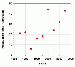
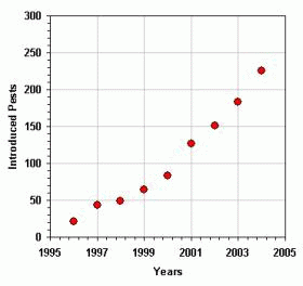
In spite of efforts done by IPPC and by many countries, in the last years, the rate of introduction of quarantine pests is increasing as can be seen in Figure 1 ([1])¹ Probably these figures underestimate the real number of introduced pests, but they clearly show a trend to increase.


Figure 1. Number of new occurrences of pest. A - Introduction rate of new pests per year. B - Accumulated number of introduced pests [1].

What worries more are that the rate of pest introduction (Fig. 1A) is growing and that the number of introduced pests seems to be exponentially increasing (Fig. 1B). The question that naturally arises from the analysis of the graph is: how can we revert the growing tendency of pest introductions?

Considering that is not acceptable to increase barriers to trade, the reduction in the rate of pest introduction could only be achieved increasing the technical capacity of the countries.

This can be shown through a conceptual model of the Global Phytosanitary System, as presented in Figure 2, and explained by the following hypotheses:

1.An increase in the intensity of the international trade tends to increase the rate of introduction of quarantine pests;

2.When the number of introduced pest increases, the cost of commodity production would also increase (after a few years time delay, because new pest management techniques will have to be applied and also the crop yield would be reduced). Higher production cost and lost of yield implies in higher prices, what put pressure to slow down the rate of international trade;

3.On the other side, when the introduced pests quantity increases, the number of phytosanitary requirements will decrease, which would speed up the international trade rate by removing trade barriers;

4.There is a "natural" build rate of the technical capacity of the countries. However the increase of the international trade intensity tends to speed up the technical capacity build rate. This is because the countries need to defend from the growing phytosanitary risk associated with trade increase. An increase in the pest introduction rate has the same effect in the build rate of the technical capacity.

5.Improved phytosanitary requirements would be developed and applied when the technical capacity is increased. This would increase the biosecurity and, as a consequence, decrease the pest introduction rate. Also, better phytosanitary requirements imply in the removal of those requirements that are not technically justified. This would help to increase the trade intensity by removing unjustified barriers.

6.The increase in the people's international transport rate shall also be considered in the system. It will cause an increase in the pest introduction rate.

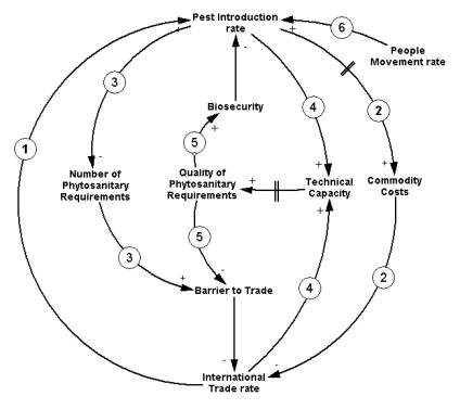
Figure 2. Conceptual model of the Global Phytosanitary System (causal loops diagram)

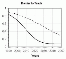
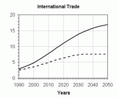
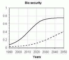
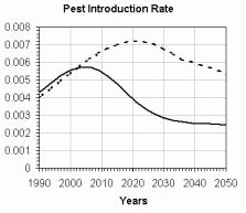
A simulation model derived from the conceptual model generates some interesting figures. We simulated two scenarios: use of 10% of the potential build of the technical capacity of the countries (dot line) and use of 90% of this potential build (continuous line). The results are presented in Figure 3.



Figure 3. Outputs from de Global Phytosanitary System model. The scales on the Y-axis are relative. Continuous line: 90% of the potential build of the technical capacity used; dot line: 10% of the potential build of the technical capacity used.

It is clearly displayed in Figure 3 the urgent need to improve the technical capacity of the countries, which implies that not only is necessary to increase the use of the available quantitative methods for phytosanitary management but also that there is a need to develop new methodologies.

In recent years, the evolution of phytosanitary approaches for the management of pest risk has led to the recognition of a rationale: if you decrease the number of fertile pest individuals in a commodity to a pre-established number assessed through risk analysis, then you will decrease the risk of establishment of this pest to an acceptable level. A considerable effort and significant progress have been made through the application of this rationale to understanding options for achieving a desired level of quarantine security. This has opened the door for expanding the understanding and use of many important concepts for risk management, including:

Pest Free Areas (places and sites of production) - a risk management option based upon a sound pest risk assessment coupled with satisfactory evidence of effective, on-going surveillance and exclusion measures to maintain such areas pest free [2].

Systems Approaches - consecutive phytosanitary measures are used to decrease the number of fertile pest individuals in a commodity.

Alternative Treatment Efficacy - where the percentage of the pest population that has to be killed is variable, depending mainly on the initial infestation level and on the characteristics of the pest and of the commodity.

Maximum Pest Limits (especially for fruit flies) has developed as "the maximum number of immature fruit flies that may be present in consignments imported during a specific time to a specific location" (see [3] and [2] for a deeper discussion on these concepts).

These initiatives demonstrate a trend toward exploring and applying more systematic approaches to evaluating (and justifying) the phytosanitary measures. Yet a common understanding of the range of possible quantitative methodologies and the development and routine use of appropriate methodologies to evaluate and compare the risk mitigation measures is far from being well developed in the phytosanitary community.

2. Acceptable Level of Risk

As there is no a risk definition in the FAO glossary, we will adopt a commonly accepted definition [4]² where risk is the product of the consequences of an event by the probability of it occurrence:

Risk = Consequences * Probability of occurrence 1

In the phytosanitary context risk would be:

Risk = Potential Economic Impact * Probability of Introduction 2

In this context “Introduction” means the entry and establishment of a pest. However, the probability can be expressed as the time lag between expected occurrences of the event. If the probability of introduction is a per year probability then we can express the risk as:

With equation 2 or 3 we can apply the Iso-Risk concept proposed by [5] and expressed in Figure 4.

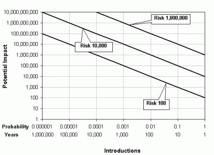
Figure 4. Iso-Risk lines (graph in log scale).

Each line is an iso-risk line, where the combination of Potential Impact and Probability of Introduction is constant. Each one could represent the Acceptable Levels of Risk (ALR) for different countries. Notice that a pest with high introduction probability and low potential impact could put the same risk that a pest with low introduction probability and high potential impact.

The main point to note at this stage is that although countries have the sovereign right to choose their ALR. It is difficult to understand what this means, unless it is expressed quantitatively (equations 2 or 3). This is consistent with the principle of transparency.

If a pest presents a risk greater than the ALR, there are two ways to decrease it. Either the Potential Impact is decreased or the Introduction Probability is decreased (or both).

Although there are ways to decrease the potential economical impact, as to begin cropping resistant varieties or to develop and apply contention plans, for instance, this paper will keep the focus in the reduction of the Introduction Probability.

If the country choose an ALR and have an estimate of the Potential Economic Impact, then for each pest can be calculated the acceptable Introduction Probability, as shown in equation 4. This is essential to support the choice of a risk management strategy, as will be discussed in the next section.

3. Probability of Introduction

From the field in one country to establishment in another country there is a chain of events that reduces the pest prevalence in one consignment of a plant or plant product, as illustrated in Figure 5.

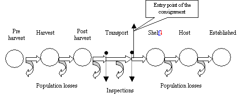
Figure 5. Population losses in the production/commercialization chain

For phytosanitary purposes, it is convenient to have a holistic approach to this system. For example, a post-harvest treatment with a known mortality rate has no meaning if we do not know the initial prevalence in the treated consignment, because we don’t know how many individuals will survive. Also, the design of an inspection system could be optimized only if we know the probabilities associated with pest entry and establishment. It is not logical to design a very sensitive, expensive inspection system to detect a very low prevalence if the pest has a poor chance to become established.

The establishment of a pest has essentially two components:

the number of pest individuals in that enters the country (consignment size * prevalence), and

the probabilities of establishment of the pest.

The entry of a pest does not mean introduction (establishment). Many factors, as described in [6] could interact to allow, or not, the establishment, as in the following examples:

probability of pest surviving existing pest management procedures;
probability of transfer to a suitable host;
probability of the environment be suitable in the PRA area, etc.

Equation 5 estimates the expected number of establishments:

Expected Introductions = Entered x Probability of Establishment 5

Entered is the number of individuals that enters into the country (consignment size times prevalence). Note that Probability of Establishment, in equation 5, is the probability of one single individual establishment, while Probability of Introduction in equations 2, 3 and 4 is the probability of ingress and establishment of one population.

To calculate the necessary efficacy of any phytosanitary measure, it is required the estimate of the number of individuals that could enter the country without resulting in establishment, considering the chosen protection level. For that it is necessary to calculate the introduction probability resulting from the individuals that enter, and also considering the establishment probability of the pest. There are equations for estimates of this probability, as a function of the entered individuals, of the pest prevalence and of the establishment probability [7]:

However as the introduction probability can also be estimated through equation 5 (because the values of expected establishments are almost the same to the introduction probability, when the values are low) this equation will be used, to keep the simplicity of this work.

Now it is possible to join equation 4 and 5 according to the following expression:

We can plot now the iso-introduction line in function of the probability of establishment and of the number of entered individuals, as shown in Figure 6.

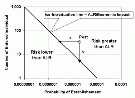
Figure 6. Iso-introduction line in relation to the number of entered individuals and the probability of a single individual establishment. In this graph the iso-introduction line is set to 0.00001 what means that the chosen ALR is 100.000 smaller than de Economic Impact. The line represents cases where

Entered Individual * Probability of Establishment = ALR/Economic Impact (Probability of Introduction).

In Figure 6, a pest is represented by the dot. As this pest is above the iso-introduction line, it has a risk greater than the ALR. To decrease its risk we have to either (a) decrease the number of entered individual; (b) decrease the probability of establishment or (c) detect consignments with larger prevalence than the acceptable (or any a, b and c combination).

Note that the lines a and b represents the necessary efficacy of equivalent measures. Note also that a and b have the same size but that any other line from the pest to the iso-introduction line is shorter than a and b. This means that when two measures are applied the combined efficacy can be lower than the efficacy of a single measure.

Example 1
Data:
Acceptable Level of Risk: US$ 1,000
Potential Economic Impact: US$ 10,000,000
Consignment size: 10,000 units
Expected Infestation Level in the consignment: 0.005 (0.5%)
Pest Establishment Probability: 0.00001

Results:

Acceptable Probability of Introduction (eq. 4) = 1,000/10,000,000 = 0.0001

Acceptable number of entered individuals (eq. 7): = 0.0001/0.00001 = 10

Expected number of entered individuals(eq. 5) = 10,000*.005 = 50 individuals

Conclusions:

Consignments of the product could be accepted if:

1. It is feasible to apply an inspection plan to detect 0.1% of infestation level

2. The infestation level in the consignment could be decreased to less than 0.1%

3. The pest establishment probability could be decreased to less than 0.000002

4. Phytosanitary Measures (PMs)

The phytosanitary measures can be grouped according to their strategy:

Group 1. Reduction of the pest population in the consignment (prevalence)

The strategy of this group is to reduce the population of the pest in the consignment and consequently, to reduce the possibility of establishment. This can be achieved by treatments or other procedures.

Pre Harvest (treatment in the field, pest free area, place or site of production, testing, etc)
Harvest (removal of infested products, inspection for selection, stage of ripeness/maturity, etc)
Post Harvest (handling, chemical/physical treatment, etc)
Shipping and distribution (volume, transport environment, in transit or on arrival treatment, limits on distribution, etc.)
Pest Free Areas (sites and places of production)

Group 2. Reduction of the probabilities of establishment

The strategy of the second group of PMs is to reduce the probabilities of establishment and so reduce the probability of introduction. This group includes measures using import management:

Frequency of importation
Season timing
Port of entry
Restriction on the end use

Group 3. Detection of infested consignments

The strategy of measures of the third group is to detect the consignments that present infestation (prevalence) above an established threshold. After the detection, the destruction, re-export or another PM of the other groups (treatment, restriction of the end use) can be applied. The following measures fall into this group:

Inspection
Testing
Post-entry quarantine.

Most of these measures are well studied and applied. There are, however, few points that deserve additional consideration.

4.1 Reduction of the population of the pest in the consignment (prevalence)

Decreasing the number of entered individuals has been the main strategy used in the past and present. The main quantitative application widely used by the phytosanitary community in the past is the probit 9 approach. It was proposed more than 65 years ago as the basis for measuring the efficacy of treatments for fruit flies [8]. The general rationale behind the probit 9 approach is very simple and straightforward: if you kill a very high percentage (99.9968 %) of the pest population then you will decrease the chance of pest establishment to zero (or very close to zero). This rationale assumes a worst-case scenario and results in a high-kill treatment requirement that may not be technically justified based on pest prevalence.

However it is interesting to note that the countries usually request the application of specific phytosanitary measures, but they don't requires maximum population thresholds. According to the preceding paragraph the number of expected establishments is directly proportional to the population entered. The efficacy of a chemical treatment, for instance, has no meaning, if the initial population size (prevalence) is unknown and consequently the number of survivals is also unknown.

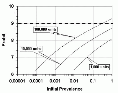
Figure 7. Necessary treatment efficacy (probit) to reduce the survivors to one individual, as a function of the initial prevalence in the product, for different consignment sizes. The dashed line represents probit 9 mortality.

Figure 7 shows that the only cases that requires probit 9 to achieve a resultant population of one individual is the ones that have an initial prevalence of 0.31 (31% infection rate) or greater and the consignment size is 100,000 units or greater. All the other combinations need inferior probit. The excess mortality rate that would be attained with probit 9 in the other cases do not lead to additional safety and is expensive, could reduce the shelf-life of the product and increase the residuals concentration (Fig. 7).

Also the probit 9 approach has been criticized, in particular because: "While probit 9 was clearly designed to reduce the prevalence of pests by a predictable amount, it does not account for other variables contributing to pest risk. Natural survival rates, the likelihood of infestation, and the colonization potential of the pest are a few of the more important risk based considerations that are ignored by a direct estimation of mortality such as probit 9. Process parameters such as pre-shipment cultural practice, packing and shipping procedures, and distribution times or areas, are not considered when mortality is the sole criterion for determining quarantine security [2].

Note that the required probit can be estimated with equation 8 (from equation 7) and is represented by line b in Fig 6.

In reducing the prevalence there are cost issues that need to be considered. The cost to develop and apply phytosanitary measures usually increases with the efficacy of the measures, while the use of measures with low efficacy could imply in lost of market opportunity and increased cost of opportunity lost. Figure 8 represents the relation between these costs and the composed cost.

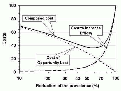
Figure 8. Cost/Benefit analysis of the phytosanitary measures to reduce prevalence.

Figure 8 shows that above certain level it is not economically viable to increase the efficacy of measures to reduce prevalence. In such cases, it will be important to evaluate the possibility to use other procedures to reduce de probability of introduction.

4.2 Reduction of the probability of establishment

Although it is relatively easy to calculate the required efficacy of phytosanitary measures to reduce the prevalence is quite more complicated to do estimates of the probability of establishment of pest populations, entered in a new environment.

The establishment probability almost always depends on the size of entered population. It is interesting to note the observations of [9]: Founder populations are typically small and consequently are at great risk of extinction. Generally, the smaller the founder population, the less likely is establishment. Though many scientists have referred to a “minimum viable population” there is rarely a distinct threshold. Instead it is more realistic to consider the probability of establishment as being a continuous function of the initial population size. This function reflects many characteristics of the species, such as its intrinsic rate of reproduction, mate location abilities, and genetic diversity.

This is in agreement with the statement of Dr. Alexei Sharov (Virginia Polytechnic Institute and State University - personal communication), who said that: “… in many cases, the dispersal pattern and the probability of finding a mate are critical for pest establishment. Insects that mate before dispersal have a higher probability of establishment. In the destination area, the initial population numbers are extremely low. So if insects disperse first, then they will probably never find a mate. This is true even for insects with very sensitive pheromone communication mechanisms (e.g. gypsy moth)”.

In 1981 it was proposed [10] the concept of Minimum Viable Population (MVP): An MVP for any given species in any given habitat is the smallest isolated population having a 99% chance of remaining extant for 1000 years despite the foreseeable effects of demographic, environmental, and genetic stochasticity, and natural catastrophes.

Lately this concept gave origin to the Population Viability Analysis (PVA) methodology that consists of estimating the probability of a population of a specified size that will persist for a specified length of time. The topic of PVA has become very popular, with two recent books [11, 12] providing extensive coverage of the topic.

PVA is usually developed through probabilistic simulation models. Although models for PVA have been developed for populations of vertebrates, they could also be used for invertebrates, especially for those that don’t have very high fertility. Deterministic and stochastic models are playing an increasing role in population management studies. Although most of the phytosanitary community is not extensively using tools like this, they could have usefulness and immediate application. As example, the program VORTEX³ [13]is probably the most widely used generic PVA model currently available. It was originally designed for modeling mammal populations, but is also suitable for modeling birds and some reptiles, invertebrates and fish populations. The program is individual-based and incorporates environmental and demographic stochasticity, inbreeding depression, metapopulations, catastrophes, and some density-dependence functions. The program also allows for simulation of harvesting from the population and supplementation (i.e. introducing translocated individuals to the population).

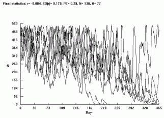
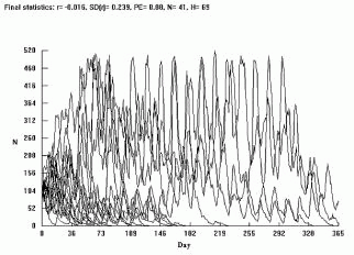
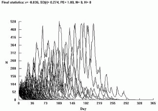
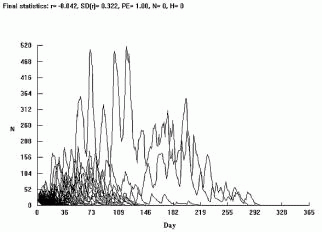
To show the relation between the population size and the probability of establishment, we have run few examples in VORTEX, using insect pest data, as is shown in Figure 9.

Figure 9. Vortex outputs of an insect pest population development, considering different initial population’s size. A - 500 individual; B - 200 individual; C - 100 individual and D - 50 individuals.

As can be noted from Figure 9 the pest will not establishes if the initial population is below 200 individuals. The results show also that the probability of population extinction is 0.29 for an initial population of 500 individual; 0.88 for an initial population of 200 individuals and of 1.0 for initial populations of 100 and 50 individuals.

This type of information could support the estimates of the number of individuals of the pest that could enter the country and, consequently, to supply the technical justification for the development of safe phytosanitary requirements. However, the necessary data should be reliable and not always they are available.

Consignment Size x Frequency of Importations

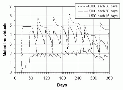
This is an issue that is not very often considered as a risk management procedure. However, the probability of establishment can be greatly changed by frequency and size of consignments. We had investigated this through a simulation model representing consignments size equivalent to 100 units per day and a delivery prevalence of 1% insect pest larvae. The larval mortality is 60%; the pupae mortality is 50% and 50% of the adults mate. The longevity of the mated adult is around 55 days. Figure 10 presents results of tree scenarios (a) 1,500 units consignments arriving each 15 days; (b) 3,000 units consignments arriving each 30 days and (c) 6,000 units arriving each 60 days.

Figure 10. Simulation of the development of a population of insects in consignments arriving in the delivery site at different time intervals. Note that these results are regarding a fictitious pest.

The graph in Figure 10 shows that the number of mated individual in the delivery site can be reduced, through the reduction of the size of each consignment and reduction of the time interval between the consignments, keeping constant the yearly amount of the imported product. In spite of this measured being of difficult practical application, it could represent the difference among the establishment or not of the pest.

Port of Entry

The establishment probability is a function of the founder population as well as environmental conditions. Some techniques used in the study of population ecology could be used also to support the choice of the risk management strategies. As an example, Figure 11 [14] below shows a monthly graph of the humidity versus temperatures in two locations in Brazil. The dashed square represents the zone of optimum development for Ceratitis capitata ⁴(16-32^oC and 65-75% RH) as found elsewhere in the literature.

The graph shows that in Curitiba (temperate south Brazil) the environmental conditions are sub-optimum all year around, while in Fortaleza (tropical north Brazil) there are favorable conditions from September to February. Although it does not allow for any inference on the probability of establishment, the use of spatial models could be a tool to evaluate the reduction of the probabilities as function of environmental conditions.

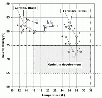
Figure 11. Climogram (Temperature x Relative Humidity) for Fortaleza and Curitiba, Brazil and zone of optimum development for Ceratitis capitata (dashed square).

The country could permit the importation entering in Fortaleza only from March to August, or only accept Curitiba as the entry port. This measure could reduce the introduction probability to the acceptable level of risk, as shown by line a in Figure 6.

There is commercial software, like CLIMEX⁵, for modeling species responses to climate that are been used for quarantine purposes.

4.3 Detection of non-compliant consignments

In Section 3 it was shown that the number of expected establishments is directly proportional to the number of entered pests and to the probability of establishment. The number of entered pests can be decreased by decreasing the infection rate in the consignments or by detecting consignments with prevalence above the accepted one.

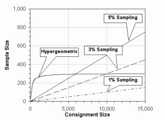
The number of samples to be taken from a consignment shall be estimated according to the hypergeometric distribution (see draft ISPM on Inspection Methodology). Schilling⁶ proposed an algebraic equation that approximates the true hypergeometric distribution. From this approximation we can estimate the number of samples required to detect a specific infection rate:

where CL is the confidence level of the sampling and Detection level is the minimum prevalence to be detected. Using the data from Example 1, in page 7, where the consignment size is 10,000 units and the required detection level is 0.001 (0.1%) then the sample size would be 2,589 units for a confidence level of 0.95 and of 3,690 units for 0.99-confidence level.

The general relation between Detection Level, Confidence Level and Sample size is presented in Figure 12.

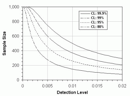
Figure 12. Sample size as function of the detection level, according to the hypergeometric distribution. The graph shows lines of four confidence levels (CL). The graph presents the sample size for a consignment of 1,000 units.

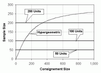
Although the hypergeometric distribution supplies the technical bases for a safe sampling, it cannot be feasible for very low detection levels, because the number of units to be sampled would be very high, as can be seen in the Figure 12.

Figure 13. A. Comparison of hypergeometric sampling with constant size sampling; B. Comparison of hypergeometric sampling with percent sampling. The graphs were draw considering a detection level of 0.1% and a confidence level of 95%.

It is interesting to note that the sampling system used for many countries is based upon the use of constant size sampling or sampling of a percentage of the consignment. However, as shown in Figure 13, these systems use either smaller or larger number of samples than the necessary. In the first case the safety of the inspection is reduced and in the second case there is unnecessary resources expenditure.

As the probability of the inspection to fail is given by 1 –Confidence Level, it can be calculated from equation 9, accordingly:

With the above equation and the introduction probability, calculated through equation 6, it is possible to verify that a prevalence range exists where the introduction probability is larger (Fig. 14).

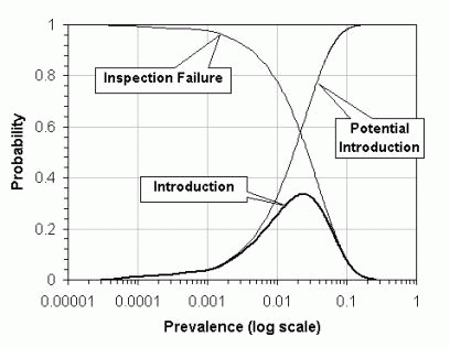
Figure 14. Probabilities of inspection failure, potential introduction and introduction as a function of prevalence in the consignment (consignment size= 1000, sample size= 25, probability of establishment= 0.04)

In this Figure, Potential Introduction means the introduction probability without consideration of the inspection process and Introduction is the probability of introduction after the consignment pass through inspection. The Figure shows that when the prevalence is low the probability of detection of an infected consignment is also low (if the sampling size is kept constant). However, when the prevalence increases the probability of detection increases (decreasing the probability of inspection failure). As the probability of introduction (before inspection) increase with the prevalence, the probability of introduction after inspection is bell shaped with a maximum around prevalence of 2%. It is important to note also that, if the prevalence increases, the trade would be unviable because the number of refused consignments would be very high.

5. Summarizing

The flowchart for the application of the concepts discussed in this paper is shown in the Figure 15. The process begins calculating the Acceptable Probability of Introduction, through the Acceptable Level of Risk (ALR) and of the potential Economical Impact (EI), with the equation 4. Then, with the equations 5 or 6, and using specific data of the pest and shipment, the Expected Probability of Introduction is calculated. If the expected probability is smaller than the acceptable one, then ALR is attained and the trade could start. Otherwise another measures should be found, either to decrease the prevalence of the pest or its establishment probability. It could also be requested smaller consignments. If the expected probability of introduction is above, but very close to the acceptable probability, the country could rely in its detection system. In this case it could be expected a larger number refused consignments.

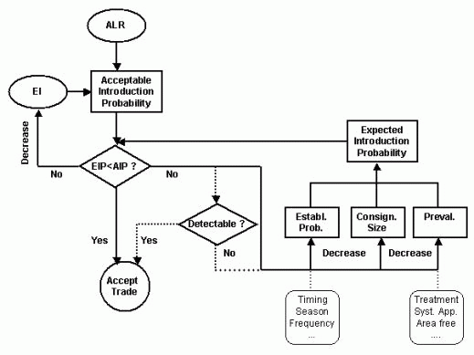
Figure 15. Conceptual flowchart of the establishment of a phytosanitary requirement.

Acknowledgments

We thank to Dr. Ron A Sequeira for the invitation to present this paper in the International Conference on SPS Risk Assessment Methodology. We also thank to Dr. Raul Valle for reviewing the manuscript.This work was accomplished with the supports of the Cocoa Research Center (CEPEC/CEPLAC, Brazil).

6. References

1.EPPO - European and Mediterranean Plant Protection Organization. Reporting Service. 1996-2004.

2. Liquido, N.J., R.L. Griffin, and K.W. Vick (eds.) 1997. Quarantine security for commodities: current approaches and potential strategies. Proceedings of Joint Workshops of the Agricultural Research Service and the Animal and Plant Health Inspection Service, June 5-9 and July 31-August 4, 1995. USDA, ARS, 1996-04, 56 pp.

3. Bartlett, P.W., G.R. Chaplin, and R.J. Van Velsend (eds.). 1996. Plant Quarantine Statistics. A Review. Proceedings of an International Workshop. Sydney, Australia - December 1995. HRDC, 93 pp.

4. Bigsby, H. and J. Crequer. 1996. Conceptual model for the management of pest risk. Statistics in Ecology and Environmental Monitoring, Dunedin, June 1996, pp. 7-16.

5. Bigsby, H. and C. Whyte. 2001. Quantifying Phytosanitary Barriers to Trade. In.: Hooker, N. and E. Murano (Eds.). Interdisciplinary Food Safety Research, CRC Press, pp. 69-85.

6. International Plant Protection Convention/FAO. 2001. Pest risk analysis for quarantine pests. International standards for phytosanitary measures. Publication n. 11, 27 pp.

7. Baker, R.T., J.M. Cowley and D.S. Harte. 1993. Pest risk assessment. Lynfield Plant Protection Centre Publications, New Zealand, N^o. 1, 12 pp.

8. Baker, A.C. 1939. The basis for treatment of products where fruit flies are involved as a condition for entry into the United States. USDA Circ. 551.

9. Liebhold, A.M., W.L. Macdonald, D. Bergdahl, and V.C. Mastro. 1995. Invasion by Exotic Forest Pests: A Threat to Forest Ecosystems. Forest Science Monographs 30.49 pp.

10. Shaffer, M.L. 1981. Minimum population size for species conservation. Bioscience 31:131-134.

11. Beissinger, S.R., and D.R. McCullough, editors. 2002. Population viability analysis. University of Chicago Press, Chicago, Illinois, USA. 577 pp.

12. Morris, W.F., and D.F. Doak. Quantitative conservation biology: theory and practice of population viability analysis. Sinauer Associates, Sunderland, Massachusetts, USA. 480 pp.

13. Lacy, R.C. 1993: Vortex: a computer simulation model for population viability analysis. Wildlife Research 20: 45–65.

14. Araújo, K.R.P. 2000.Modelo matemático para simular a aplicação da técnica do inseto estéril e etapas de implementação de um programa de controle da mosca do mediterrâneo. PhD thesis, CENA/USP, 2001.

FOOTNOTES

[1] The data were computed by counting the number of “new record”, “first record”, “first findings”, “first detection” and “first occurrence” in the index of the EPPO Service Reporting publication from 1996 to 2004.

² We suggest also the reading of the Thomas Cool’s paper “Proper definitions for Risk and Uncertainty” that can be found in the Society for Risk Analysis website: http://econwpa.wustl.edu:8089/eps/get/papers/9902/9902002.html

³http://www.vortex9.org/vortex.html

⁴Ceratitis capitata is not a quarantine pest for Brazil. It is used here only as an example.

⁵http://www.ento.csiro.au/climex/climex.html

⁶http://www-ist.massey.ac.nz/61325/sg/chap4-5.htm